Uses for Superconductors
Magnetic-levitation is an application where superconductors perform extremely well. Transport vehicles such as trains can be made to "float" on strong superconducting magnets, virtually eliminating friction between the train and its tracks. Not only would conventional electromagnets waste much of the electrical energy as heat, they would have to be physically much larger than superconducting magnets. A landmark for the commercial use of MAGLEV technology occurred in 1990 when it gained the status of a nationally-funded project in Japan. The Minister of Transport authorized construction of theYamanashi Maglev Test Line which opened on April 3, 1997. In December 2003, the MLX01 test vehicle (shown above) attained an incredible speed of 361 mph (581 kph).
Although the technology has now been proven, the wider use of MAGLEV vehicles has been constrained by political and environmental concerns (strong magnetic fields can create a bio-hazard). The world's first MAGLEV train to be adopted into commercial service, a shuttle in Birmingham, England, shut down in 1997 after operating for 11 years. A Sino-German maglev is currently operating over a 30-km course at Pudong International Airport in Shanghai, China. The U.S. plans to put its first (non-superconducting) Maglev train into operation on a Virginia college campus. Click this link for a website that listsother uses for MAGLEV.

MRI of a human skull.
An area where superconductors can perform a life-saving function is in the field of biomagnetism. Doctors need a non-invasive means of determining what's going on inside the human body. By impinging a strong superconductor-derived magnetic field into the body, hydrogen atoms that exist in the body's water and fat molecules are forced to accept energy from the magnetic field. They then release this energy at a frequency that can be detected and displayed graphically by a computer. Magnetic Resonance Imaging (MRI) was actually discovered in the mid 1940's. But, the first MRI exam on a human being was not performed until July 3, 1977. And, it took almost five hours to produce one image! Today's faster computers process the data in much less time.
The Korean Superconductivity Group within KRISS has carried biomagnetic technology a step further with the development of a double-relaxation oscillation SQUID (Superconducting QUantum Interference Device) for use in Magnetoencephalography. SQUID's are capable of sensing a change in a magnetic field over a billion times weaker than the force that moves the needle on a compass (compass: 5e-5T, SQUID: e-14T.). With this technology, the body can be probed to certain depths without the need for the strong magnetic fields associated with MRI's.
Probably the one event, more than any other, that has been responsible for putting "superconductors" into the American lexicon was the Superconducting Super-Collider project planned for construction in Ellis county, Texas. Though Congress cancelled the multi-billion dollar effort in 1993, the concept of such a large, high-energy collider would never have been viable without superconductors. High-energy particle research hinges on being able to accelerate sub-atomic particles to nearly the speed of light. Superconductor magnets make this possible. CERN, a consortium of several European nations, is doing something similar with its Large Hadron Collider (LHC) recently inaugurated along the Franco-Swiss border.
Other related web sites worth visiting include the proton-antiproton collider page at Fermilab. This was the first facility to use superconducting magnets. Get information on the electron-proton collider HERA at the German lab pages of DESY (with English text). And Brookhaven National Laboratory features a page dedicated to its RHIC heavy-ion collider.
Electric generators made with superconducting wire are far more efficient than conventional generators wound with copper wire. In fact, their efficiency is above 99% and their size about half that of conventional generators. These facts make them very lucrative ventures for power utilities. General Electrichas estimated the potential worldwide market for superconducting generators in the next decade at around $20-30 billion dollars. Late in 2002 GE Power Systems received $12.3 million in funding from the U.S. Department of Energy to move high-temperature superconducting generator technology toward full commercialization.
Other commercial power projects in the works that employ superconductor technology include energy storage to enhance power stability. American Superconductor Corp. received an order from Alliant Energy in late March 2000 to install a Distributed Superconducting Magnetic Energy Storage System (D-SMES) in Wisconsin. Just one of these 6 D-SMES units has a power reserve of over 3 million watts, which can be retrieved whenever there is a need to stabilize line voltage during a disturbance in the power grid. AMSC has also installed more than 22 of its D-VAR systems to provide instantaneous reactive power support.
The General Atomics/Intermagnetics General superconducting
Fault Current Controller, employing HTS superconductors.
Hypres Superconducting Microchip,
Incorporating 6000 Josephson Junctions.
The National Science Foundation, along with NASA and DARPA and various universities, are currently researching "petaflop" computers. A petaflop is a thousand-trillion floating point operations per second. Today's fastest computers have only recently reached "petaflop" speeds - quadrillions of operations per second. Currently the fastest is the U.S. Department of Energy "Sequoia" Supercomputer, operating at 16.32 petaflops per second. The fastest single processor is a Lenslet optical DSP running at 8 teraflops. It has been conjectured that devices on the order of 50 nanometers in size along with unconventional switching mechanisms, such as the Josephson junctions associated with superconductors, will be necessary to achieve the next level of processing speeds. TRW researchers (now Northrop Grumman) have quantified this further by predicting that 100 billion Josephson junctions on 4000 microprocessors will be necessary to reach 32 petabits per second. These Josephson junctions are incorporated into field-effect transistors which then become part of the logic circuits within the processors. Recently it was demonstrated at the Weizmann Institute in Israel that the tiny magnetic fields that penetrate Type 2 superconductors can be used for storing and retrieving digital information. It is, however, not a foregone conclusion that computers of the future will be built around superconducting devices. Competing technologies, such as quantum (DELTT) transistors, high-density molecule-scale processors , and DNA-based processing also have the potential to achieve petaflop benchmarks.
In the electronics industry, ultra-high-performance filters are now being built. Since superconducting wire has near zero resistance, even at high frequencies, many more filter stages can be employed to achive a desired frequency response. This translates into an ability to pass desired frequencies and block undesirable frequencies in high-congestion rf (radio frequency) applications such as cellular telephone systems. ISCO International andSuperconductor Technologies are companies currently offering such filters.
Superconductors have also found widespread applications in the military. HTSC SQUIDS are being used by the U.S. NAVY to detect mines and submarines. And, significantly smaller motors are being built for NAVY ships using superconducting wire and "tape". In mid-July, 2001, American Superconductor unveiled a 5000-horsepower motor made with superconducting wire (below). An even larger 36.5MW HTS ship propulsion motor was delivered to the U.S. Navy in late 2006
The newest application for HTS wire is in the degaussing of naval vessels. American Superconductor has announced the development of asuperconducting degaussing cable. Degaussing of a ship's hull eliminates residual magnetic fields which might otherwise give away a ship's presence. In addition to reduced power requirements, HTS degaussing cable offers reduced size and weight.
The military is also looking at using superconductive tape as a means of reducing the length of very low frequency antennas employed on submarines. Normally, the lower the frequency, the longer an antenna must be. However, inserting a coil of wire ahead of the antenna will make it function as if it were much longer. Unfortunately, this loading coil also increases system losses by adding the resistance in the coil's wire. Using superconductive materials can significantly reduce losses in this coil. The Electronic Materials and Devices Research Group at University of Birmingham (UK) is credited with creating the first superconducting microwave antenna. Applications engineers suggest that superconducting carbon nanotubes might be an ideal nano-antenna for high-gigahertz and terahertz frequencies, once a method of achieving zero "on tube" contact resistance is perfected.
The most ignominious military use of superconductors may come with the deployment of "E-bombs". These are devices that make use of strong, superconductor-derived magnetic fields to create a fast, high-intensity electro-magnetic pulse (EMP) to disable an enemy's electronic equipment. Such a device saw its first use in wartime in March 2003 when US Forces attacked an Iraqi broadcast facility.
A photo of Comet 73P/Schwassmann-Wachmann 3, in the act of disintegrating ,
taken with the European Space Agency S-CAM.
Among emerging technologies are a stabilizing momentum wheel (gyroscope) for earth-orbiting satellites that employs the "flux-pinning" properties of imperfect superconductors to reduce friction to near zero. Superconducting x-ray detectors and ultra-fast, superconducting light detectors are being developed due to their inherent ability to detect extremely weak amounts of energy. Already Scientists at the European Space Agency (ESA) have developed what's being called the S-Cam, an optical camera of phenomenal sensitivity (see above photo). And, superconductors may even play a role in Internet communications soon. In late February, 2000, Irvine Sensors Corporation received a $1 million contract to research and develop a superconducting digital router for high-speed data communications up to 160 Ghz. Since Internet traffic is increasing exponentially, superconductor technology may be called upon to meet this super need.
According to June 2002 estimates by the Conectus consortium, the worldwide market for superconductor products is projected to grow to near US $38 billion by 2020. Low-temperature superconductors are expected to continue to play a dominant role in well-established fields such as MRI and scientific research, with high-temperature superconductors enabling newer applications. The above ISIS graph gives a rough breakdown of the various markets in which superconductors are expected to make a contribution.
All of this is, of course, contingent upon a linear growth rate. Should new superconductors with higher transition temperatures be discovered, growth and development in this exciting field could explode virtually overnight.
Another impetus to the wider use of superconductors is political in nature. The reduction of green-house gas (GHG) emissions has becoming a topical issue due to the Kyoto Protocol which requires the European Union (EU) to reduce its emissions by 8% from 1990 levels by 2012. Physicists in Finland have calculated that the EU could reduce carbon dioxide emissions by up to 53 million tons if high-temperature superconductors were used in power plants.
The future melding of superconductors into our daily lives will also depend to a great degree on advancements in the field of cryogenic cooling. New, high-efficiency magnetocaloric-effect compounds such as gadolinium-silicon-germanium are expected to enter the marketplace soon. Such materials should make possible compact, refrigeration units to facilitate additional HTS applications. Stay tuned !
Magnetic-levitation is an application where superconductors perform extremely well. Transport vehicles such as trains can be made to "float" on strong superconducting magnets, virtually eliminating friction between the train and its tracks. Not only would conventional electromagnets waste much of the electrical energy as heat, they would have to be physically much larger than superconducting magnets. A landmark for the commercial use of MAGLEV technology occurred in 1990 when it gained the status of a nationally-funded project in Japan. The Minister of Transport authorized construction of theYamanashi Maglev Test Line which opened on April 3, 1997. In December 2003, the MLX01 test vehicle (shown above) attained an incredible speed of 361 mph (581 kph).
Although the technology has now been proven, the wider use of MAGLEV vehicles has been constrained by political and environmental concerns (strong magnetic fields can create a bio-hazard). The world's first MAGLEV train to be adopted into commercial service, a shuttle in Birmingham, England, shut down in 1997 after operating for 11 years. A Sino-German maglev is currently operating over a 30-km course at Pudong International Airport in Shanghai, China. The U.S. plans to put its first (non-superconducting) Maglev train into operation on a Virginia college campus. Click this link for a website that listsother uses for MAGLEV.
MRI of a human skull.
An area where superconductors can perform a life-saving function is in the field of biomagnetism. Doctors need a non-invasive means of determining what's going on inside the human body. By impinging a strong superconductor-derived magnetic field into the body, hydrogen atoms that exist in the body's water and fat molecules are forced to accept energy from the magnetic field. They then release this energy at a frequency that can be detected and displayed graphically by a computer. Magnetic Resonance Imaging (MRI) was actually discovered in the mid 1940's. But, the first MRI exam on a human being was not performed until July 3, 1977. And, it took almost five hours to produce one image! Today's faster computers process the data in much less time.
The Korean Superconductivity Group within KRISS has carried biomagnetic technology a step further with the development of a double-relaxation oscillation SQUID (Superconducting QUantum Interference Device) for use in Magnetoencephalography. SQUID's are capable of sensing a change in a magnetic field over a billion times weaker than the force that moves the needle on a compass (compass: 5e-5T, SQUID: e-14T.). With this technology, the body can be probed to certain depths without the need for the strong magnetic fields associated with MRI's.
Probably the one event, more than any other, that has been responsible for putting "superconductors" into the American lexicon was the Superconducting Super-Collider project planned for construction in Ellis county, Texas. Though Congress cancelled the multi-billion dollar effort in 1993, the concept of such a large, high-energy collider would never have been viable without superconductors. High-energy particle research hinges on being able to accelerate sub-atomic particles to nearly the speed of light. Superconductor magnets make this possible. CERN, a consortium of several European nations, is doing something similar with its Large Hadron Collider (LHC) recently inaugurated along the Franco-Swiss border.
Other related web sites worth visiting include the proton-antiproton collider page at Fermilab. This was the first facility to use superconducting magnets. Get information on the electron-proton collider HERA at the German lab pages of DESY (with English text). And Brookhaven National Laboratory features a page dedicated to its RHIC heavy-ion collider.
Electric generators made with superconducting wire are far more efficient than conventional generators wound with copper wire. In fact, their efficiency is above 99% and their size about half that of conventional generators. These facts make them very lucrative ventures for power utilities. General Electrichas estimated the potential worldwide market for superconducting generators in the next decade at around $20-30 billion dollars. Late in 2002 GE Power Systems received $12.3 million in funding from the U.S. Department of Energy to move high-temperature superconducting generator technology toward full commercialization.
Other commercial power projects in the works that employ superconductor technology include energy storage to enhance power stability. American Superconductor Corp. received an order from Alliant Energy in late March 2000 to install a Distributed Superconducting Magnetic Energy Storage System (D-SMES) in Wisconsin. Just one of these 6 D-SMES units has a power reserve of over 3 million watts, which can be retrieved whenever there is a need to stabilize line voltage during a disturbance in the power grid. AMSC has also installed more than 22 of its D-VAR systems to provide instantaneous reactive power support.
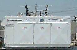
The General Atomics/Intermagnetics General superconducting
Fault Current Controller, employing HTS superconductors.
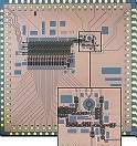
Hypres Superconducting Microchip,
Incorporating 6000 Josephson Junctions.
The National Science Foundation, along with NASA and DARPA and various universities, are currently researching "petaflop" computers. A petaflop is a thousand-trillion floating point operations per second. Today's fastest computers have only recently reached "petaflop" speeds - quadrillions of operations per second. Currently the fastest is the U.S. Department of Energy "Sequoia" Supercomputer, operating at 16.32 petaflops per second. The fastest single processor is a Lenslet optical DSP running at 8 teraflops. It has been conjectured that devices on the order of 50 nanometers in size along with unconventional switching mechanisms, such as the Josephson junctions associated with superconductors, will be necessary to achieve the next level of processing speeds. TRW researchers (now Northrop Grumman) have quantified this further by predicting that 100 billion Josephson junctions on 4000 microprocessors will be necessary to reach 32 petabits per second. These Josephson junctions are incorporated into field-effect transistors which then become part of the logic circuits within the processors. Recently it was demonstrated at the Weizmann Institute in Israel that the tiny magnetic fields that penetrate Type 2 superconductors can be used for storing and retrieving digital information. It is, however, not a foregone conclusion that computers of the future will be built around superconducting devices. Competing technologies, such as quantum (DELTT) transistors, high-density molecule-scale processors , and DNA-based processing also have the potential to achieve petaflop benchmarks.
In the electronics industry, ultra-high-performance filters are now being built. Since superconducting wire has near zero resistance, even at high frequencies, many more filter stages can be employed to achive a desired frequency response. This translates into an ability to pass desired frequencies and block undesirable frequencies in high-congestion rf (radio frequency) applications such as cellular telephone systems. ISCO International andSuperconductor Technologies are companies currently offering such filters.
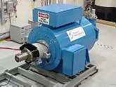
Superconductors have also found widespread applications in the military. HTSC SQUIDS are being used by the U.S. NAVY to detect mines and submarines. And, significantly smaller motors are being built for NAVY ships using superconducting wire and "tape". In mid-July, 2001, American Superconductor unveiled a 5000-horsepower motor made with superconducting wire (below). An even larger 36.5MW HTS ship propulsion motor was delivered to the U.S. Navy in late 2006
In the electronics industry, ultra-high-performance filters are now being built. Since superconducting wire has near zero resistance, even at high frequencies, many more filter stages can be employed to achive a desired frequency response. This translates into an ability to pass desired frequencies and block undesirable frequencies in high-congestion rf (radio frequency) applications such as cellular telephone systems. ISCO International andSuperconductor Technologies are companies currently offering such filters.
Superconductors have also found widespread applications in the military. HTSC SQUIDS are being used by the U.S. NAVY to detect mines and submarines. And, significantly smaller motors are being built for NAVY ships using superconducting wire and "tape". In mid-July, 2001, American Superconductor unveiled a 5000-horsepower motor made with superconducting wire (below). An even larger 36.5MW HTS ship propulsion motor was delivered to the U.S. Navy in late 2006
The newest application for HTS wire is in the degaussing of naval vessels. American Superconductor has announced the development of asuperconducting degaussing cable. Degaussing of a ship's hull eliminates residual magnetic fields which might otherwise give away a ship's presence. In addition to reduced power requirements, HTS degaussing cable offers reduced size and weight.
The military is also looking at using superconductive tape as a means of reducing the length of very low frequency antennas employed on submarines. Normally, the lower the frequency, the longer an antenna must be. However, inserting a coil of wire ahead of the antenna will make it function as if it were much longer. Unfortunately, this loading coil also increases system losses by adding the resistance in the coil's wire. Using superconductive materials can significantly reduce losses in this coil. The Electronic Materials and Devices Research Group at University of Birmingham (UK) is credited with creating the first superconducting microwave antenna. Applications engineers suggest that superconducting carbon nanotubes might be an ideal nano-antenna for high-gigahertz and terahertz frequencies, once a method of achieving zero "on tube" contact resistance is perfected.
The most ignominious military use of superconductors may come with the deployment of "E-bombs". These are devices that make use of strong, superconductor-derived magnetic fields to create a fast, high-intensity electro-magnetic pulse (EMP) to disable an enemy's electronic equipment. Such a device saw its first use in wartime in March 2003 when US Forces attacked an Iraqi broadcast facility.
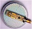
A photo of Comet 73P/Schwassmann-Wachmann 3, in the act of disintegrating ,
taken with the European Space Agency S-CAM.
Among emerging technologies are a stabilizing momentum wheel (gyroscope) for earth-orbiting satellites that employs the "flux-pinning" properties of imperfect superconductors to reduce friction to near zero. Superconducting x-ray detectors and ultra-fast, superconducting light detectors are being developed due to their inherent ability to detect extremely weak amounts of energy. Already Scientists at the European Space Agency (ESA) have developed what's being called the S-Cam, an optical camera of phenomenal sensitivity (see above photo). And, superconductors may even play a role in Internet communications soon. In late February, 2000, Irvine Sensors Corporation received a $1 million contract to research and develop a superconducting digital router for high-speed data communications up to 160 Ghz. Since Internet traffic is increasing exponentially, superconductor technology may be called upon to meet this super need.
According to June 2002 estimates by the Conectus consortium, the worldwide market for superconductor products is projected to grow to near US $38 billion by 2020. Low-temperature superconductors are expected to continue to play a dominant role in well-established fields such as MRI and scientific research, with high-temperature superconductors enabling newer applications. The above ISIS graph gives a rough breakdown of the various markets in which superconductors are expected to make a contribution.
All of this is, of course, contingent upon a linear growth rate. Should new superconductors with higher transition temperatures be discovered, growth and development in this exciting field could explode virtually overnight.
Another impetus to the wider use of superconductors is political in nature. The reduction of green-house gas (GHG) emissions has becoming a topical issue due to the Kyoto Protocol which requires the European Union (EU) to reduce its emissions by 8% from 1990 levels by 2012. Physicists in Finland have calculated that the EU could reduce carbon dioxide emissions by up to 53 million tons if high-temperature superconductors were used in power plants.
The future melding of superconductors into our daily lives will also depend to a great degree on advancements in the field of cryogenic cooling. New, high-efficiency magnetocaloric-effect compounds such as gadolinium-silicon-germanium are expected to enter the marketplace soon. Such materials should make possible compact, refrigeration units to facilitate additional HTS applications. Stay tuned !


 the equation relate to each other. For instance, the equation suggests that for objects moving around circles of different radius in the same period, the object traversing the circle of larger radius must be traveling with the greatest speed. In fact, the average speed and the radius of the circle are directly proportional. A twofold increase in radius corresponds to a twofold increase in speed; a threefold increase in radius corresponds to a three--fold increase in speed; and so on. To illustrate, consider a strand of four LED lights positioned at various locations along the strand. The strand is held at one end and spun rapidly in a circle. Each LED light traverses a circle of different radius. Yet since they are connected to the same wire, their period of rotation is the same. Subsequently, the LEDs that are further from the center of the circle are traveling faster in order to sweep out the circumference of the larger circle in the same amount of time. If the room lights are turned off, the LEDs created an arc that could be perceived to be longer for those LEDs that were traveling faster - the LEDs with the greatest radius. This is illustrated in the diagram at the right.
 velocity vector is directed in the same direction that the object moves. Since an object is moving in a circle, its direction is continuously changing. At one moment, the object is moving northward such that the velocity vector is directed northward. One quarter of a cycle later, the object would be moving eastward such that the velocity vector is directed eastward. As the object rounds the circle, the direction of the velocity vector is different than it was the instant before. So while the magnitude of the velocity vector may be constant, the direction of the velocity vector is changing. The best word that can be used to describe the direction of the velocity vector is the word

 always acts downward; its magnitude can be found as the product of mass and the acceleration of gravity (
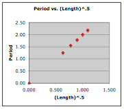
 A simple pendulum consists of a relatively massive object hung by a string from a fixed support. It typically hangs vertically in its equilibrium position. The massive object is affectionately referred to as thependulum bob. When the bob is displaced from equilibrium and then released, it begins its back and forth vibration about its fixed equilibrium position. The motion is regular and repeating, an example of periodic motion. Pendulum motion was introduced
 In physical situations in which the forces acting on an object are not in the same, opposite or perpendicular directions, it is customary to resolve one or more of the forces into components. This was the practice used in the analysis of sign hanging problems and inclined plane problems. Typically one or more of the forces are resolved into perpendicular components that lie along coordinate axes that are directed in the direction of the acceleration or perpendicular to it. So in the case of a pendulum, it is the gravity force which gets resolved since the tension force is already directed perpendicular to the motion. The diagram at the right shows the pendulum bob at a position to the right of its equilibrium position and midway to the point of maximum displacement. A coordinate axis system is sketched on the diagram and the force of gravity is resolved into two components that lie along these axes. One of the components is directed tangent to the circular arc along which the pendulum bob moves; this component is labeled Fgrav-tangent. The other component is directed perpendicular to the arc; it is labeled Fgrav-perp. You will notice that the perpendicular component of gravity is in the opposite direction of the tension force. You might also notice that the tension force is slightly larger than this component of gravity. The fact that the tension force (Ftens) is greater than the perpendicular component of gravity (Fgrav-perp) means there will be a net force which is perpendicular to the arc of the bob's motion. This must be the case since we expect that
 ng the arc towards C, then B and then A. As it does, there is a leftward restoring force opposing its motion and causing it to slow down. So as the displacement increases from D to A, the speed decreases due to the opposing force. Once the bob reaches position A - the maximum displacement to the right - it has attained a velocity of 0 m/s. Once again, the bob's velocity is least when the displacement is greatest. The bob completes its cycle, moving leftward from A to B to C to D. Along this arc from A to D, the restoring force is in the direction of the motion, thus speeding the bob up. So it would be logical to conclude that as the position decreases (along the arc from A to D), the velocity increases. Once at position D, the bob will have a zero displacement and a maximum velocity. The velocity is greatest when the displacement is least. The animation at the right (used with the permission of Wikimedia Commons; special thanks to Hubert Christiaen) provides a visual depiction of these principles. The acceleration vector that is shown combines both the perpendicular and the tangential accelerations into a single vector. You will notice that this vector is entirely tangent to the arc when at maximum displacement; this is consistent with the force analysis discussed above. And the vector is vertical (towards the center of the arc) when at the equilibrium position. This also is consistent with the force analysis discussed above.